neural concept learning
If I trained a neural net, will it learn concepts like a Bayesian?
This is an overview of my final project for MIT 9.660: Computational Cognitive Science. For more details, check out the report and the code repository.
Introduction
How do humans make inferences from limited amounts of observation data? This is a big question that concept learning aims to answer.
Some important works in this field study a toy example called the Number game
Let’s have a try! Take a moment to look at these numbers…
What do you notice? Chances are, you might infer a hypothesis that this program is the “powers of two” concept. But, how did we infer this? And in particular, why did we infer specifically this hypothesis, and not “powers of two except 32”, or any one of the myriad other hypotheses that could work? This was a central question explored in some of the most original works in concept learning.
One explanation is the Bayesian model. This model says that, in a universe of numbers \(\mathcal U\), before even observing the set of numbers \(D\subseteq\mathcal U\), we already have a prior on how likely different concepts \(C\) are: we might think that “powers of two” is a lot more likely than “powers of two except 32”. This prior constrains the generalization that we infer. Mathematically, this is formulated as Bayes’ theorem:
\[\Pr\left[C\mid D\right]\propto\Pr\left[D\mid C\right]\Pr\left[C\right]\]We can use these posteriors to infer the probability that a number belongs to an unknown concept:
\[\Pr\left[x\in C\mid D\right]=\sum_{C_i:\,x\in C_i}\Pr\left[C_i\mid D\right]\]These are great ideas that have been shown to work very well, but let’s focus on a different question: what if our priors were wrong? What if they were so wrong that the true concept had a prior probability of zero, and the observation had zero likelihood under all hypotheses in our hypothesis space? Then, our Bayesian model would encounter a “division by zero”, which means it’s doomed…
Model architecture
Having a model break down like this really isn’t good. After all, real humans don’t usually send a SIGFPE when encountering an unexpected input.
Let’s break free of this problem by trying something completely different: a neural network! The main strength of a model like this is that we no longer have to impose such a strict Bayesian structure. This means we can count on it to always output something, even if we’re in a zero-prior or zero-likelihood scenario.
However, its greatest strength is also its greatest weakness. While the model is guaranteed to output something, there’s no longer any guarantee that it’ll output anything meaningful, because the model doesn’t have to be Bayesian! As we’ll soon see though, this effect turns out to be… not too bad.
Let’s concretize the idea a bit.
We will use Attention
We implement this model with softmax attention,
but be aware that \(f(\cdot\mid D)\) isn’t actually a probability distribution!
We can train it using Adam
Let’s see how Bayesian this model is! And then, let’s also see what it does when the observation doesn’t work with our hypothesis space.
Experiment
To keep things tractable, we’ll make our universe \(\mathcal U\) the set of integers between 1 and 30, and our space of concepts will consist of a few instances of “multiples of \(m\)” and “intervals between \(p\) and \(q\)”. We first train our model with a large set of generated observations, with varying latent dimension \(n\).
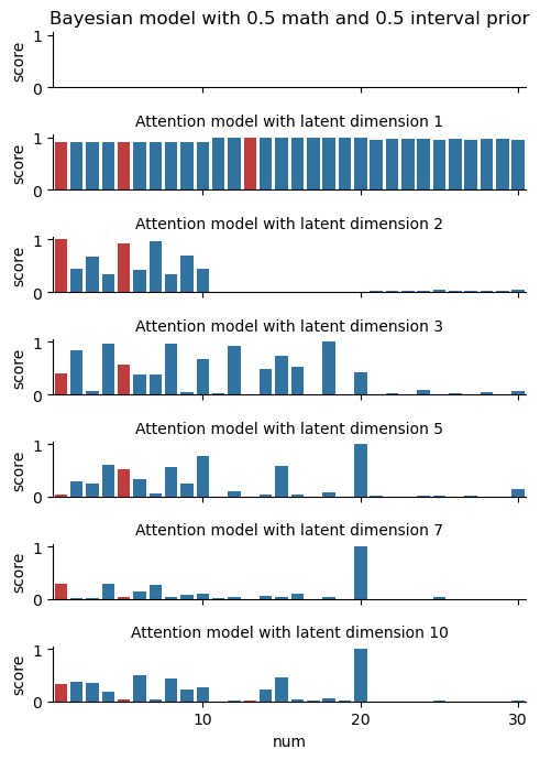
Here’s what our predictions look like when we evaluate our model on two different observation sets \(D=\left\{12\right\}\) and \(D=\left\{12,16\right\}\). We also include a reference Bayesian model to use as a baseline.
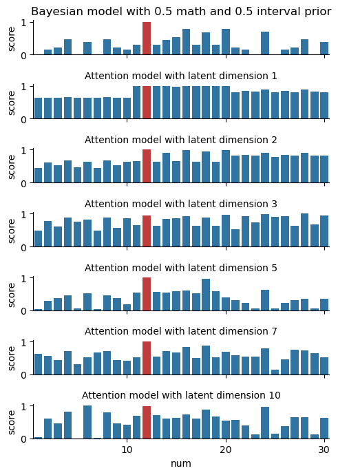
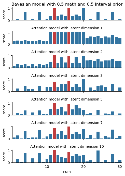
We can see the model learn more as the latent dimension increases: it starts with the “intervals” at \(n=1\), then adds on “parity” at \(n=2\), and so on. By \(n=5\), it looks a lot like the Bayesian model! In comparing the left and right figures, the model also responds to the additional observation point in a reasonable way. This is not by accident… but more on this in the Theory section later.
We also sent out a survey asking real humans to play some rounds of the Number game. Out of sheer curiosity, we trained a model using this data, although the results were far from stellar. Humans aren’t perfect Bayesians, after all — see for yourself below.
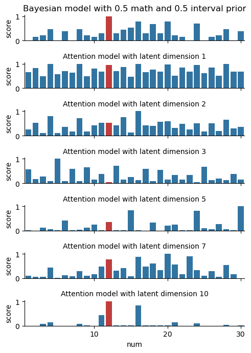
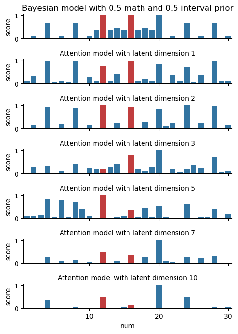
Back to our original question: what does our (original) model do when given nonsense input? We played a little trick on our human volunteers and unknowingly gave them some observations \(D\) that were entirely random numbers. Will our model be able to explain how the humans responded?
Well, there’s still some work to do. On the one hand, the diagram below shows that our model will indeed produce an output on the nonsense data, while the Bayesian model fails entirely. However, a quantitative evaluation shows that the model achieves far better loss on the “regular” data than on the nonsense data; for example, at \(n=5\) the respective losses are 3.550 compared with 4.688. The model also predicts some very strange things when given a nonsense observation; its out-of-sample generalization is not that good.
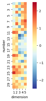
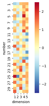
To gain some ideas on what the model’s actually doing, we can take a look at the learned embeddings \(k\) and \(q\). These are illustrated above: each dimension appears to have learnt some combination of concepts, with some such as “between 11 and 20” and “even numbers” standing out. While the model itself isn’t perfect, we can glean some interpretability from the model weights!
Theory
The results suggest that a neural network can mimic some of the behaviors of a Bayesian agent. This is actually by design: our network architecture makes this possible!
Let’s take a quick moment to fill in a gap about how the Bayesian agent works:
what is the likelihood term \(\Pr\left[D\mid C\right]\)?
It was found that the one below works well,
and if you think about it, it also makes a lot of sense
Now let’s imagine a toy scenario. Say there’s two concepts: \(C_1\subset C_2\subseteq\mathcal U\), and say they have equal priors. Suppose you observe a set \(D\subseteq C_1\). Then, for \(x\in C_1\) and \(y\in C_2\setminus C_1\):
\[\begin{aligned} \frac{\Pr\left[x\in C\mid D\right]}{\Pr\left[y\in C\mid D\right]} &= \frac{\Pr\left[D\mid C_1\right]+\Pr\left[D\mid C_2\right]}{\Pr\left[D\mid C_2\right]} \\ &= \frac{\left|C_1\right|^{-\left|D\right|}+\left|C_2\right|^{-\left|D\right|}}{\left|C_2\right|^{-\left|D\right|}} \\ &= 1+\left(\frac{\left|C_2\right|}{\left|C_1\right|}\right)^{\left|D\right|} \label{eq:posterior-odds-bayesian} \end{aligned}\]On the other hand, suppose the neural model \(f\) has \(n=2\) and learns embeddings \(q_z,k_z\in\mathbb R^2\) such that for some constant \(c>1\),
\[(q_z)_i = (k_z)_i = \begin{cases} \sqrt{\ln c} & z\in C_ i \\ 0 & z\not\in C_ i \end{cases}\]Then,
\[\begin{aligned} \frac{f(x\mid D)}{f(y\mid D)} &= \exp\left(\sum_{z\in D}\left\langle q_x,k_z\right\rangle-\left\langle q_y,k_z\right\rangle\right) \nonumber\\ &= \exp\left(\left|D\right|\ln c\right) \nonumber\\ &= c^{\left|D\right|} \end{aligned}\]For the appropriate value of \(c\), this is not too far from the Bayesian model! In fact, as \(\left|D\right|\to\infty\) (our observation set gets large), our neural model can behave just like the Bayesian!
So, perhaps it’s not all that surprising that our model is able to look Bayesian. What’s impressive, though, is that it was able to learn this type of behavior, despite the analysis above being restricted to toy scenarios such as this. Of course, as the experiments show, there’s still room for improvement!
Implications
We’ve proposed modelling the Number game using a self-attention network. We’ve learnt a few things about it from our experiments:
- It looks like it can behave like a Bayesian on in-sample concepts.
- Its embeddings can give us some amount of interpretability into the model’s behavior.
- Its out-of-sample generalization is not quite up-to-standard yet.
The most exciting part is that the architecture enables Bayesian-like behavior. What remains to be discovered is how to enforce that little bit more structure, to enable better out-of-sample generalization, while not being so strict as to fail as a perfect Bayesian would.